Attention
You might be wondering if this article can possible contain anything new for you. You already studied the illustrated and annotated Transformer, the original paper and everything from GPT-1-2-3 to BERT and beyond. Well, if you have, it could indeed be that there is nothing fundamentally new for you to be found here. But the goal to weave all this information into one coherent story and provide further context across dimensions and domains with a focus on attention itself instead of the scaffolding erected around it referred to as The Transformer has the potential to further clarify and solidify some of these truly interesting and general concepts.
Notation
Our detailed explanation of the attention mechanism begins with some math which will subsequently be visualized to build an intuitive understanding. A quick word on notation: The attention equation makes use of scalars, vectors and matrices. We will use lowercase letters $x$, bold lowercase letters $\boldsymbol{x}$ and uppercase letters $W$ for these entities respectively. A great way to visualize scalars, vectors and matrices is to represent them by colored squares, where the number of squares represents the dimensionality and the shade of the color in each square represents the magnitude of the value at this position from small, bright values to large, dark values as shown below.
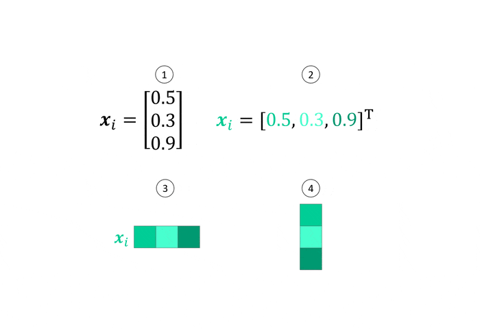
Most illustrations in this article are animated. Simply hover over them with your mouse (or tap on them) to activate the animation.
The basic attention equation
Making use of our notation, the basic attention equation can be written as
\[\boldsymbol{y}_j = \sum_{i=1}^Nw_{ij}\boldsymbol{x}_i\]So what’s happening here? In a nutshell: The output of the attention operation $\boldsymbol{y}_j$ is a weighted sum of the inputs $\boldsymbol{x}_i$. The inputs are the set elements introduced in the previous article, for example words, pixels or points in 3D space. They are usually vectors, where the dimensions, referred to as (input) features, can represent various properties like RGB color channels or XYZ Euclidean coordinates. Words are somewhat special in this regard, as they don’t have any intrinsic features and are therefore commonly represented by a large vector with values encoding their semantics computed from their co-occurrence with other words which is called an embedding1.
The dot product and softmax
What are those weights $w_{ij}$ then and how are they determined? Though we employ attention in the deep learning domain, in it’s most basic form, it actually doesn’t contain any learnable parameters. Instead, the weights are computed from the inputs using the dot product as similarity measure: $w_{ij}=\boldsymbol{x}_i^T\boldsymbol{x}_j$. To understand how this works and why it makes sense, let’s take a look at the visualization below (reminder: hover over or tap on the image to activate the animation).
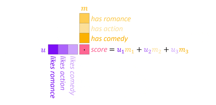
The two vectors $\boldsymbol{u}$ and $\boldsymbol{m}$ represent the movie preferences of a user and the movie content respectively with three features each. Now, taking the dot product, we get a score representing the match between user and movie. Note that this takes into account both the magnitude of the values, as multiplying large values results in a large increase of the score, as well as the sign. Imagine a scale between $-1$ and $1$ where the former represent strong dislike (or weak occurance in case of the movie vector) and the latter a strong inclination (or strong occurance). Now, given a user who dislikes action and a movie with little action, the score will still be high as both negative signs cancel out, which is exactly what we want. To make those weights more interpretable and prevent the output from becoming excessively large, we can squish all weights $\boldsymbol{w}_j={w_{ij}}_{i=1}^N$ to fall between $0$ and $1$ using the softmax function which is reminiscent of its application on the logits in classification tasks. We can think of the resulting normalized weight vector as a categorical probability distribution over the inputs where high probability is assigned to inputs with strong similarity2 and attention itself as expected value of the inputs.
Animated attention
Once all weights are computed, we multiply them with their corresponding inputs and sum them up to obtain the $j^{th}$ output which, as stated before, is simply a weighted sum of the inputs3. The computation graph below visualizes the entire process.
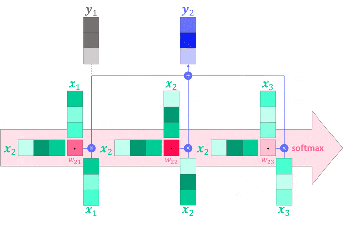
As in the dot product example, think of the transposed vectors (the horizontal ones) as individual users and the vertical ones as movies. The outputs would then represent something akin to an ideal movie, one for each user, stitched together from the three individual movies on offer.
Following Feynmans “What I cannot create, I do not understand” let’s also quickly implement basic attention in Python:
import numpy as np

# Inputs: Three RGB-D pixels (RGB colors and depth)
x_1, x_2, x_3 = [np.random.randint(0, 255, 4) for _ in range(3)]
x_i = [x_1, x_2, x_3]

# First, we compute all "raw" attention weights w_ij
w_1j = [x_1.dot(x) for x in x_i]
w_2j = [x_2.dot(x) for x in x_i]
w_3j = [x_3.dot(x) for x in x_i]

# Then we pass them through the softmax function
def softmax(x):
    e_x = np.exp(x - np.max(x))
    return e_x / e_x.sum()

w_1j = softmax(w_1j)
w_2j = softmax(w_2j)
w_3j = softmax(w_3j)

# Finally, the output is the weighted sum of the inputs
y_1 = np.sum([w * x for w, x in zip(w_1j, x_i)], axis=0)
y_2 = np.sum([w * x for w, x in zip(w_2j, x_i)], axis=0)
y_3 = np.sum([w * x for w, x in zip(w_3j, x_i)], axis=0)
Queries, keys and values
But wait, we aren’t actually dealing with different entities like users and movies in this basic formulation of attention, as all three vectors involved—two of which are used to compute the weight and the remaining one as part of the weighted sum—stem from the same set $X$. This also means that output $\boldsymbol{y}_1$ will be dominated by input $\boldsymbol{x}_1$ as the dot product between two identical vectors is usually large (after all, they are as similar as it gets). To deal with these issues, we can try to make the attention computation more versatile and expressive through the introduction of three learnable parameter matrices $W^Q$, $W^K$ and $W^V$. Through multiplication with the inputs $\boldsymbol{x}$ we obtain three distinct vectors for the three roles on offer namely the query $\boldsymbol{q}$, key $\boldsymbol{k}$ and value $\boldsymbol{v}$.
\[\boldsymbol{q}=W^Q\boldsymbol{x} \quad \boldsymbol{k}=W^K\boldsymbol{x} \quad \boldsymbol{v}=W^V\boldsymbol{x}\]The basic attention equation therefore becomes:
\[\boldsymbol{y}_j = \sum_{i=1}^Nw_{ij}\boldsymbol{v}_i \\ w_{ij}=\boldsymbol{q}_i^T\boldsymbol{k}_j\]Returning to our running example, the query takes on the role of the user, asking the question: “Which movies match my taste?” while the key encodes the movies content and the value represents the movie itself. Using this updated definition, the computation performed by the attention operation can be visualized as follows.
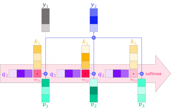
We can add these changes to our basic attention implementation with a few lines of code:
import numpy as np

# Inputs: Three RGB-D pixels (RGB colors and depth)
x_i = [np.random.randint(0, 255, 4) for _ in range(3)]

# Define query, key and value weight matrices
# In reality, they would be learned using backprop
W_Q = np.random.random([4, 3])
W_K = np.random.random([4, 3])
W_V = np.random.random([4, 3])

# Compute queries, keys and values
q_1, q_2, q_3 = [x.dot(W_Q) for x in x_i]
k_1, k_2, k_3 = [x.dot(W_K) for x in x_i]
v_1, v_2, v_3 = [x.dot(W_V) for x in x_i]
v_i = [v_1, v_2, v_3]

# Compute all "raw" attention weights w_ij
# This time using queries and keys
w_1j = [q_1.dot(k) for k in [k_1, k_2, k_3]]
w_2j = [q_2.dot(k) for k in [k_1, k_2, k_3]]
w_3j = [q_3.dot(k) for k in [k_1, k_2, k_3]]

# Then we pass them through the softmax function
def softmax(x):
    e_x = np.exp(x - np.max(x))
    return e_x / e_x.sum()

w_1j = softmax(w_1j)
w_2j = softmax(w_2j)
w_3j = softmax(w_3j)

# Finally, the output is the weighted sum of the values
y_1 = np.sum([w * v for w, v in zip(w_1j, v_i)], axis=0)
y_2 = np.sum([w * v for w, v in zip(w_2j, v_i)], axis=0)
y_3 = np.sum([w * v for w, v in zip(w_3j, v_i)], axis=0)
Attention as soft dictionary
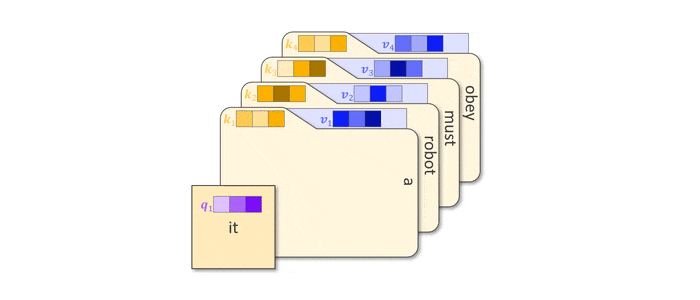
The terms key and value might remind you of dictionaries used across programming languages, where values can be stored and retrieved efficiently using a hash of the key. Indeed, such dictionaries are nothing but the digital successor of file cabinets where files (values) are stored in folders with labels (keys). Given the task to retrieve a specific file (query) you would find it by comparing the search term to all labels. Using this analogy, we can understand attention as a soft dictionary, returning every value to the extend that its key matches the query.
Parallelization using matrices
From the illustrations you might get the impression that attention is computed sequentially, one input at a time. Luckily, this is not the case when we move to matrix notation. All we need to do is to stack the (transposed) inputs $\boldsymbol{x}_i$ into an input matrix $X$ which we can than directly multiply with the query, key and value parameter matrices. As a mental aid, you could think of $X$ as a color image of dimension $32\times32\times3$ flattened to a matrix of shape $1024\times3$4.
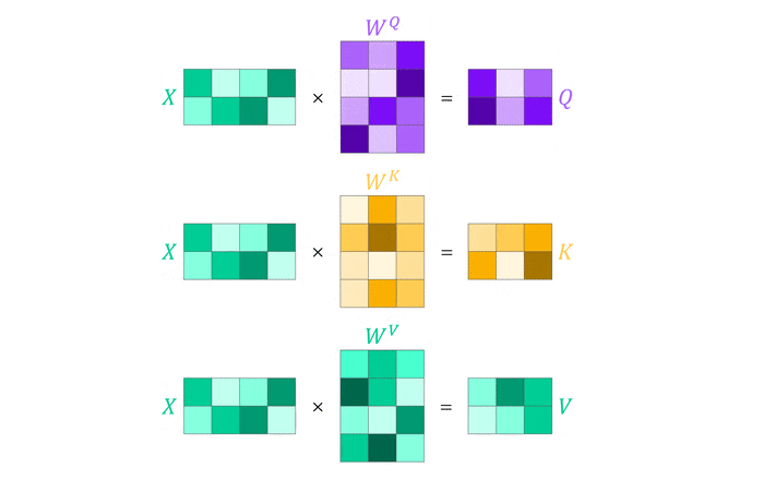
The obtained query, key and value matrices $Q$, $K$ and $V$ then simply replace the individual values in the attention equation. Note how this conveniently eliminates the need for summation, an inherent feature of matrix multiplication, and that the softmax function can be applied immediately as all weights are computed simultaneously5.

import numpy as np
from scipy.special import softmax

# Inputs: Three RGB-D pixels (RGB colors and depth)
# But this time we stack them into a matrix
x_i = [np.random.randint(0, 255, 4) for _ in range(3)]
X = np.vstack(x_i)

# Define query, key and value weight matrices
W_Q = np.random.random([4, 3])
W_K = np.random.random([4, 3])
W_V = np.random.random([4, 3])

# Compute all queries, keys and values in parallel
Q = X @ W_Q
K = X @ W_K
V = X @ W_V

# No need to compute raw attention weights
# Softmax is applied row-wise
Y = softmax(Q @ K.T, axis=1) @ V
There are three open questions before we can wrap this up: (1) What is $\sqrt{d_k}$?, (2) What about multi-head attention? and (3) How does this compare to simple fully-conntected layers and convolutions? Let’s look at these in turn.
Tempering with softmax
Dividing the values inside the softmax function by a scalar is known as tempering and the scalar is referred to as the temperature. This is often beneficial as a way of calibrating the result as squishing values into zero-one range doesn’t magically produce a proper probability distribution6. On a more practical note, dividing by $\sqrt{d_k}$ eliminates the influence of inputs with varying length7 and keeps values within the region of significant slope of the softmax function, thus preventing vanishing gradients and slow learning during training when attention is used in a deep learning context.
Multi-head attention
To understand the need for multiple heads when employing attention, let’s consider the following example.

Focusing on the word gave, our single-headed approach will place equal attention on Susan and Mary, as per the distributional hypothesis (see below), $\boldsymbol{x}_{susan}\approx\boldsymbol{x}_{mary}$ which implies $\boldsymbol{q}_{susan}\approx\boldsymbol{q}_{mary}$ bringing us to $w_{susan,mary}\approx w_{mary,susan}$.
The distributional hypothesis: You shall know a word by the company it keeps.
In other words, we can’t discern the giver from the receiver. Another way to look at this is from the output perspective, where $\boldsymbol{y}_{gave}$ will be identical for both permutations of Susan and Mary in the sentence. In other words, each individual output vector of attention is permutation invariant with respect to the inputs while the set of outputs $Y$ is permutation equivariant, meaning changing the order of the inputs will change the order of the outputs in exactly the same way. Now, this is a simple problem with a simple solution: While it is difficult to discern the function of Mary and Susan in the sentence merely from the dot product similarity of their feature vectors (that is to say, using attention) it becomes trivial when looking at their position in the sentence. In $A$ gave $B$, the name appearing before gave is always the giver while the name after it is always the receiver, which is why architectures making use of attention, like the Transformer, extend the input representation by an additional positional component (another embedding).
A more challenging problem is depicted below in the form of an ambiguous sentence which we have already encountered in the introductory article:
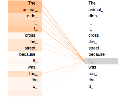
Attention weights between it and all other words in the sentence are shown where darker shades correspond to greater magnitude. The meaning of it is ambiguous, as it can correspond to animal or road. Input $\boldsymbol{x}_{it}$ only has access to a single attention weight vector $\boldsymbol{w}_{it,k}$ though, where $k$ corresponds to all other words in the sentence (or more precisly, all of their keys). Thus we can only pay attention to either animal or road but not both. Technically we could place equal weights on both, but that doesn’t help in parsing the meaning of it either. The intuitive solution is to have two attention weight vectors, encoding two different meanings of our ambiguous word. This is precisely what multi-head attention achieves.
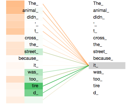
Multi-head attention is exactly like normal attention, just multiple times. Instead of a single $W^Q$, $W^K$ and $W^V$ matrix we now have $h$ of each. As this would increase the computational complexity by a factor of $h$, we divide the dimensionality of the weight matrices by this factor. Our matrices $W^Q\in\mathbb{R}^{d\times d_k}$, $W^K\in\mathbb{R}^{d\times d_k}$ and $W^V\in\mathbb{R}^{d\times d_v}$ become $h$ matrices $W_i^Q\in\mathbb{R}^{d\times d_k/h}$, $W_i^K\in\mathbb{R}^{d\times d_k/h}$ and $W_i^V\in\mathbb{R}^{d\times d_v/h}$ with inputs $\boldsymbol{x}\in\mathbb{R}^d$, queries and keys $\boldsymbol{q,k}\in\mathbb{R}^{d_k}$ and values $\boldsymbol{v}\in\mathbb{R}^{d_v}$. In practise, $d_k=d_v=d/h$ so let’s ditch $d_v$ for simplicity.
There remain two things we need to take care of. First, we don’t want to apply attention sequentially $h$ times, so we stack the $h$ weight matrices for queries, keys and values respectively and then multiply them with the inputs which results in one query, key and value vector of dimension $hd_k$ instead of $h$ each of dimension $d_k$. Second, we want the output to have the same dimensionality as the input, so we introduce a final output weight matrix $W^O\in\mathbb{R}^{hd_k\times d}$ which transforms our intermediate outputs $\boldsymbol{z}\in\mathbb{R}^{hd_k}$ into the final output $\boldsymbol{y}\in\mathbb{R}^{d_k}=\boldsymbol{z}^TW^O$. That’s quite a number of vectors, matrices and dimensions to juggle around in you head so hopefully the following visualization helps to clarify the concept.
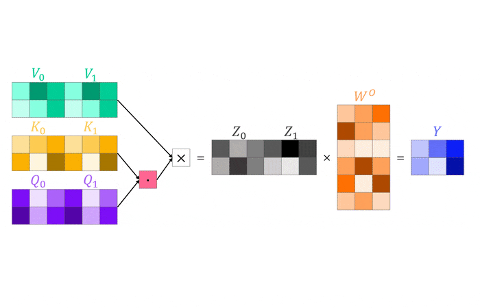
In the illustration above we have two input vectors, $\boldsymbol{x}_1$ and $\boldsymbol{x}_2$, both of size $\mathbb{R}^{4\times1}$ stacked into an input matrix (row-wise) of size $X\in\mathbb{R}^{2\times4}$. We transform the inputs using two attention heads ($h=2$) with parameter matrices $W_i^Q$, $W_i^K$ and $W_i^V$ with $i\in[1,2]$ all of size $\mathbb{R}^{4\times3}$. Through stacking of the query, key and value matrices (column-wise) from both heads we obtain three matrices of size $\mathbb{R}^{4\times6}$. We can now multiply the input matrix with the query, key and value matrices of both heads simultaneously and compute an intermediate output matrix $Z\in\mathbb{R}^{2\times6}$ using the dot product between our two-head query and key matrix and multiplying the result with our two-head value matrix. Finally, to transform the intermediate output $Z$ into the final output $Y\in\mathbb{R}^{2\times3}$, we apply the output weight matrix $W^O\in\mathbb{R}^{6\times3}$.
Putting attention into perspective
To wrap things up, let’s try to put attention into a broader context. In particular, let’s think about differences and similarities of attention to two mature building blocks of deep learning models: The fully-connected (or dense) and the convolutional layer. As both the fully-connected and the attention approach multiply the inputs with learnable weight matrices, you might wonder whether we even need both. While the input is projected once in the fully-connected case, attention projects it three times to obtain query, key and value representations. It then uses the similarity of the resulting queries and keys to construct outputs as weighted sums of inputs. This means that the activations of a fully-connected layer, i.e. the outputs prior to the non-linearity, are purely determined by the learned (fixed) weights during inference, while in attention, they are further modulated through their similarity.
In the case of convolutional layers multi-head attention can be interpreted as a generalization of discrete convolution. Given a convolutional kernel $W\in\mathbb{R}^{k\times k}$ placed on the $i^{th}$ input element we now use $h=k^2$ heads and attention weights $w_{ij}=1$ if $j=i\pm (k^2-1)/2$. This means we only consider keys which are within kernel size distance to the query where the query corresponds to the center of the kernel. With $W^V=I$ the output matrix $W^O$ then corresponds to the convolutional kernel. As the explanation is a little convoluted itself have a look at the visualization below for some intuition.

Credits
A huge thanks to Jay Alammar (The Illustrated Transformer) and Peter Bloem (Transformers from Scratch) for their excellent blog posts and videos on the subject which formed the basis of my understanding and this article. I also want to thank all researchers, authors and creators listed in the references for their great ideas and content.
References
-
Search for “word2vec” if you want further details. I recommend this blog post. ↩
-
Keep in mind though, that this is not a real probability distribution where the probability values correspond to empirical frequencies but rather a miscalibrated approximation. ↩
-
This is omitted in the basic attention equation but we will include it in the upcoming matrix notation. ↩
-
Remember, we are dealing with sets of elements, in this case pixels, which are feature vectors, in this case the RGB color values. ↩
-
Note that $QK^T$ computes a matrix of weights where each row holds the weights for the weighted sum of each output so the softmax function needs to be applied row-wise. ↩
-
Using the Bayesian interpretation of probabilities, good calibration means to be as confident or uncertain in a prediction as is warranted by the empirical frequency of being correct. Classifying an image depicting a cat with probability $0.7$ implies that, on average, $7$ out of every $10$ cat images should be classified correctly. ↩
-
The euclidean length of a vector in $\mathbb{R}^{d_k}$ with values $v$ is $\sqrt{d_k}v$. ↩